Automatic Tolerancing
The main focus of this release is rapid, automatic tolerance analysis based on the Jacobian (sensitivity matrix) of the system. Going forward, this feature will be referred to as AUTOTOL. It turns tolerance analysis from a manual, iterative process into a fast, automated, optimization-based workflow.
Listed first are the major updates in this release, followed by a brief description of the AUTOTOL feature. For a complete list of updates, please refer to the release notes in the user manual.
Updates
Basic_Consexample script has been converted to the moduleoptim.basic_cons.- A potential crash scenario related to apertures has been resolved.
- Various improvements have been made to listing functions.
- Various improvements have been made to the internal ray-tracing engine.
- An
autotolexample script has been added to demonstrate the automatic tolerancing feature.
AUTOTOL
AUTOTOL is based on the method described in the paper “Unified approach for tolerance analysis, synthesis, and compensator selection”. This post provides a brief overview of the method and its implementation in COPHASAL. Tolerances are, by definition, small limits on deviations in system parameters. Hence, their treatment falls within the linear regime. In this case, the system sensitivity matrix, also known as the Jacobian, can be used efficiently to perform tolerance analysis and synthesis. An example script, autotol, is provided to demonstrate the use of this feature.
Jacobian
An optical system can have multiple parameters with associated tolerances. Let us denote the set of system parameters by the vector $\mathbf{r}$ and the perturbations in the system parameters by the vector $\mathbf{v}$. Assume that we are interested in monitoring and controlling a set of linear quantities, $z_i$, arranged to form the vector $\mathbf{z}$, which we will refer to as the Z-vector. Then the element of the Jacobian matrix, $J_{ij}$, is the partial derivative of $z_i$ with respect to $r_j$, that is, $J_{ij}=\partial z_i/\partial r_j$. If $\mathbf{z_0}$ is the Z-vector for the nominal system, then the perturbed Z-vector can be expressed as $$ \mathbf{z} = \mathbf{z_0} + \mathbf{J}\mathbf{v} $$
Z-Vector and Performance Metric
$z_i$ can be any quantity of interest that behaves linearly with respect to small perturbations. For example, it can be the coefficients of the Zernike polynomial expansion of the wavefront across the pupil. In this case, $\mathbf{z}^\mathrm{T}\mathbf{z}$ is the wavefront variance, which is a common performance metric. Consider a Z-vector such that $$ z_i = \frac{x_i - \left<x\right>}{\sqrt{n}} $$ where $n$ is the number of rays, $x_i$ is the transverse ray position for the $i^{th}$ ray, and $\left<x\right>$ is the mean transverse ray position. The inner product of this Z-vector is the spot-size variance, that is, $\mathbf{z}^\mathrm{T}\mathbf{z} = \sigma^2$. In general, we define the performance criterion for the tolerance analysis as $$ \mathbf{z}^\mathrm{T}\mathbf{z} = w^2 \leq w^2_0 $$
Compensation and the Quadratic Form
We can select a set of compensators, whose elements are individual system parameters or linear combinations of system parameters. Let there be $N$ compensators, and let the direction of the $n$th compensator be the unit vector $\mathbf{c}^{(n)}$ and its magnitude be $\gamma^{(n)}$. Then the Z-vector for the compensated system is given by $$ \mathbf{z}=\mathbf{z_0}+\mathbf{J}\left(\mathbf{v}-\sum_{n=1}^{N}\gamma^{(n)}\mathbf{c}^{(n)}\right)=\mathbf{z_0}+\mathbf{J}\left(\mathbf{v}-\mathbf{C\Gamma}\right) $$ Here, $\mathbf{C}$ is the matrix with $N$ columns, each of which is $\mathbf{c}^{(i)}$, and $\Gamma_i=\gamma^{(i)}$. The optimal compensator magnitudes are estimated using the following equation: $$ \mathbf{\Gamma}=\mathbf{M}^{-1}\mathbf{C}^\mathrm{T}(\mathbf{J}^\mathrm{T}\mathbf{z_0}+\mathbf{D}\mathbf{v}) $$ where $\mathbf{D}=\mathbf{J}^\mathrm{T}\mathbf{J}$ and $\mathbf{M}=\mathbf{C}^\mathrm{T}\mathbf{DC}$. With this compensation applied, the residual performance metric, $w^2$, is given by the following quadratic form: $$ w^2 = \mathbf{v}^\mathrm{T}\mathbf{Q}\mathbf{v} + \mathbf{L}\mathbf{v} + b $$ where $$ \mathbf{Q} = \mathbf{D} - \mathbf{D}\mathbf{C}\mathbf{M}^{-1}\mathbf{C}^\mathrm{T}\mathbf{D} $$ $$ \mathbf{L} = 2\mathbf{z_0}^\mathrm{T}\mathbf{J}(\mathbf{I}-\mathbf{C}\mathbf{M}^{-1}\mathbf{C}^\mathrm{T}\mathbf{D}) $$ $$ b = \mathbf{z_0}^\mathrm{T}(\mathbf{I}-\mathbf{JC}\mathbf{M}^{-1}\mathbf{C}^\mathrm{T}\mathbf{J}^\mathrm{T})\mathbf{z_0} $$ and the performance criterion for tolerance analysis can be rewritten as $$ \mathbf{v}^\mathrm{T}\mathbf{Q}\mathbf{v} + \mathbf{L}\mathbf{v} + b \leq w_{0}^{2} $$
I will not go over the derivation of the above equations and other details in this post; however, a few important points are worth noting. The left-hand side of the above equation is a quadratic form in $\mathbf{v}$ and a convex function, since $\mathbf{Q}$ is a positive semidefinite matrix; that is, its eigenvalues are non-negative. The situation is summarized in the figure below for a 2D case with eigenvalues that are strictly positive. In this case, the region defined by the above inequality is an ellipsoid, as shown in the figure below. The rectangular box shown is the region in which the system perturbation vector $\mathbf{v}$ can lie, given the tolerances for the respective parameters. In higher dimensions, this rectangular box is known as an orthotope, which is a generalization of a rectangle.
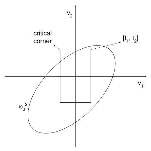
Situation described by the quadratic form in 2D, when the eigenvalues are strictly positive. The positive orthant corner vector is identified. It describes the shape of the rectangle and is defined by the tolerances for the respective parameters.
For AUTOTOL to work correctly, singular tolerances are removed from the analysis, and from the quadratic form as well. These are tolerances for parameters that have little sensitivity with respect to the performance metric and can therefore be set arbitrarily. The number of singular tolerances is affected by the compensators used.
Tolerance Synthesis and Bounds
It is important to realize that, due to convexity, if the corners of the rectangle are inside the ellipsoid, then the entire rectangle is inside the ellipsoid, and hence all possible perturbed states of the system are guaranteed to satisfy the performance criterion. However, not all corners are equally critical. In the situation shown in the figure above, the corner vector in the top-left orthant is the most critical one, since it is closest to the ellipsoid. Finding the correct orthant is not trivial; however, AUTOTOL implements a simple and effective iterative method to find the most critical corner vector.
The figure above should make it clear that, in order to synthesize the tolerances, we need to ensure that the most critical corner vector is inside or on the ellipsoid while, at the same time, the tolerances are as large as possible. One way to do this is to ensure that the corner vector lies on the ellipsoid while maximizing the area of the rectangle. In AUTOTOL, this is done by an iterative process based on the fixed-point iteration method. Interested users can refer to the autotol example script for details. Maximizing the area of the rectangle is intuitive; however, it is also possible, and often more convenient, to minimize the manufacturing cost directly. This is discussed in the next section.
After tolerance synthesis, the application of upper and lower bounds on the tolerances is straightforward. In AUTOTOL, this is done by an iterative process based on the Projection Onto Convex Sets (POCS) method.
Cost Structure
In order to minimize manufacturing cost, we first define the manufacturing cost per parameter as a function of the tolerance, $$ cost_i = \frac{\alpha_i}{t_i} $$ where $\alpha_i$ is a constant and $t_i$ is the tolerance for the $i^{th}$ parameter. The total manufacturing cost is then given by $$ cost = \sum \frac{\alpha_i}{t_i} = \mathbf{\alpha}^\mathrm{T}\mathbf{t}^{(inv)} $$ where $\mathbf{t}^{(inv)}$ is the vector of inverse tolerances. The vector $\mathbf{\alpha}$ is called the cost structure vector. The user defines the cost structure vector based on the manufacturing cost of each parameter. By default, AUTOTOL assumes $\alpha_i = 1$ for all $i$ and uses this cost function to minimize manufacturing cost while ensuring that the performance criterion is satisfied.
One free benefit of using AUTOTOL is that the final cost becomes a single number that can be used to compare different compensator configurations. This is very useful when there are multiple similar compensators to choose from.
Note that the result of AUTOTOL is a set of tolerance scale factors. That is, the final corner vector is a set of scale factors that are multiplied by the original tolerances to obtain the final tolerances. This makes the results easier to manage and interpret.
Example
For a simple example, consider a Double Gauss lens prepared for tolerance analysis. The autotol example script was run on this system. autotol uses various tolerance-analysis-specific modules and ties them together to provide a simple interface while printing diagnostic information along the way. Listed below are the main steps in the process followed by autotol after it performs some housekeeping.
- The first thing it does is estimate the Jacobian matrix. This can take a few seconds and is the only time-consuming step in the entire process. For this example, $\mathbf{J}$ had 1632 rows and 40 columns, one column for each parameter with an assigned tolerance. At this point, it also records the nominal Z-vector, $\mathbf{z_0}$.
- Next, it asks the user to define the compensator set and generates the compensator matrix, $\mathbf{C}$. In this example, the image surface was used as the only compensator.
- With the Jacobian and compensator matrix ready, it generates the quadratic form. The quadratic form of interest is defined as a class so that there can be multiple quadratic forms in an analysis, for example, one with compensators and one without compensators. The quadratic form class does the bulk of the work in AUTOTOL.
- With the help of the quadratic form, singular tolerances are identified and removed from the analysis. These parameters are not very sensitive with respect to the performance metric and can be “freely” perturbed.
- Then, based on the user-supplied performance criterion, tolerance scale factors are synthesized using an iterative method provided by the quadratic form. These are called the unbounded tolerances, and they are then adjusted to satisfy the tolerance bounds using the POCS method. These are the final bounded tolerances.
- As a sanity check, a pseudo Monte Carlo simulation is performed using the quadratic-form-based linear surrogate model to rapidly generate a large number of trials.
- Finally,
autotoloffers to apply the new tolerances to the system and prepare it for a real Monte Carlo simulation. In doing so, it scales the magnitudes of the non-singular tolerances while keeping the singular tolerances unchanged. It also freezes the system and sets the compensator parameters as variables for optimization.
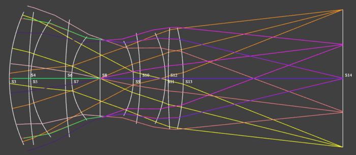
Double Gauss lens with apertures defined, additional fields defined to break symmetry, and tolerances defined.
The performance criterion was spot-size variance, with $w^2_0 = 2500 \mu m^2$, which was almost twice the nominal spot-size variance of $\mathbf{z_0}^\mathrm{T}\mathbf{z_0}$. Image-surface refocus was the only compensator used. For the upper and lower bounds, double and half of the original tolerance were used. The results of the tolerance synthesis are shown in the figure below. Note that all curvature and axial displacement tolerances were effectively made singular by the compensator choice and are not shown in the figure. Out of 40 tolerances, 18 non-singular tolerances remain.
After the most critical corner vector was found, it had to be scaled down by a factor of 0.82 to lie on the ellipsoid. This is shown by the blue curve. Results of the automatic tolerance synthesis are shown by the red curve. Although these are the unbounded tolerances, they already lie within the bounds, so the final bounded tolerances are the same as the unbounded tolerances. Tilt tolerances had to be tightened, while decenter tolerances were relaxed.
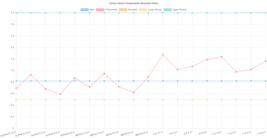
Absolute values of the corner vector components for non-singular tolerances.
Pseudo Monte Carlo Simulation
Although the primary automation in AUTOTOL is tolerance synthesis, it is also possible to perform a pseudo Monte Carlo simulation, that is, a Monte Carlo simulation using the quadratic form to leverage the surrogate linear model for speed. The object-oriented design of the quadratic form class is useful here. Given a perturbed system state vector, the compensator magnitudes are estimated using a compensated quadratic form. The final adjusted state vector is then used by the uncompensated quadratic form to estimate the performance metric.
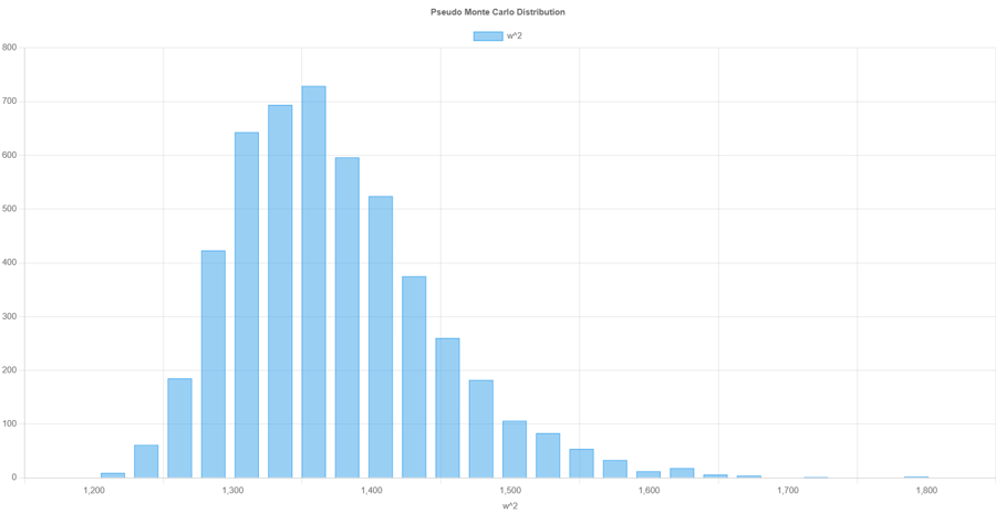
5000-trial pseudo Monte Carlo simulation results.
One thing worth noting is that, in the above results, the worst-case performance metric is about 1800, which is less than the performance criterion ($w^2_0$) of 2500. This is likely due to the fact that, even though the system state vector is equally likely to be anywhere in the orthotope, only a few corners lie on the ellipsoid, and there are many corners ($2^{18}$ in this case) to choose from.
Conclusion
The true power of AUTOTOL is most visible in demanding systems such as lithography projection lenses, high-performance microscope objectives, and similar designs, where there are many tolerances, tight performance requirements, and cost constraints. However, since it supports any Z-vector, it can be used for any system to rapidly obtain an excellent starting point for a final, full Monte Carlo simulation.