Version 1.14.32
At XLOPTIX, we wish you a very happy and prosperous new year! Special thanks to COPHASAL users for your continued support and feedback. I am pleased to announce the release of COPHASAL version 1.14.32. This release has one addition and several updates. Here we go!
Updates
scale_lens()function was not scalingTORICandQCONsurfaces, it has been fixed.Solvernow supports the operator(). Calling the solver object like a function will invoke theSolve()method. Furthermore, this way you can supply the maximum evaluations as an optional argument. For example,opt(25)is equivalent toopt:Solve()with maximum evaluations set to 25.- For optimizing the optical system, it is no longer necessary to set a cost function,
Solverwill by default use the inbuilt cost function. - The algorithm to fill the pupil of the system has been improved.
Ideal Thin Lens Surface
This surface is defined by the surface type "IDEAL". It models a thin lens that perfectly images between a given pair of conjugate planes, while obeying the sine condition. It currently supports only two parameters: effective focal length and magnification. The actual focal lengths are influenced by the index of refraction of the medium on either side of the surface. One use case of this surface is to acertain the severity of the prevailing aberrations. Here is a simple example demonstrating its use.
blank()

-- Fields
ins_fld(2, {x = 0.0, y = 15.0})

-- Sequential surfaces
set("THI S 1", 100000000000.0);

ins_surf("S 2", {type = "SPHERE", glass = "AIR", rdy = 0.0, thi = 1.0})

change_surf("S 3", "IDEAL")
set("EFL S 3", 1, 1)

set_stop(3)

showlens({fan=1})
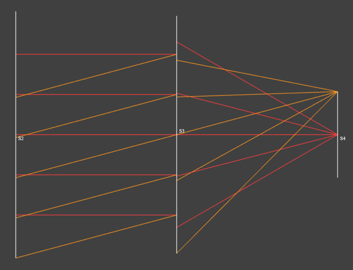
Showing an ideal thin lens surface (S3) with magnification of 0.0 (object at infinity) and effective focal length of 1 mm.
The disjointed rays at the ideal lens surface are a consequence of the fact that due to the sine condition, ray heights are maintained on the principal spheres, not on principal planes.
Matrix Operations, Regression Analysis Example
I had indicated in the previous post that matrix operations will be discussed in the upcoming post. I have decided to discuss matrix operations in multiple posts. In this post, I will demonstrate how to perform linear regression analysis using the matrix operations available in COPHASAL.
Noisy Data Generation
We will start by generating some noisy data points that we will later fit a line to. The following code snippet generates N data points along the line y = m*x + c, with noise added to the y values.
local m = 1.5;      local c = 1.0 -- y = m * x + c
local xmin = 0.0;   local xmax = 10.0
local N = 100;      local noise_level = 2.0

-- Generate noisy data points
local dp = {}
local step = (xmax - xmin) / (N - 1)
for i = 0, N - 1 do
    local x = xmin + i * step
    local noise = (math.random() * 2 - 1) * noise_level
    local y = m * x + c + noise
    table.insert(dp, {x, y})
end
This noisy line is labeled as “Data” in the plot below. Next, we will fit a line to these data points.
Linear Regression Using Matrix Operations
To perform linear regression, we will use the least squares method as described in the following code snippet.
-- Least Squares Fit
--[[
x_i * m + c = y_i, for all i
X * M = Y, where M = [m, c]'; X_i = [x_i, 1]; Y_i = y_i
M = (X^T * X)^-1 * X^T * Y
--]]

local data = Matrix.new(dp) -- data_i = [x_i, y_i]
local temp = Matrix.new(2, 1)
temp[1][1] = 1
local X = data * temp -- X_i = x_i
X:concat(Matrix.new(N, 1)+1, true) -- X_i = [x_i, 1]

temp[1][1] = 0
temp[2][1] = 1
local Y = data * temp -- Y_i = y_i

-- A crucial step, without clone() Xt is same as X
local Xt = X:clone():transpose()

local M = (Xt * X)^-1 * Xt * Y
The resulting matrix M contains the slope and intercept of the best-fit line. Let us look at some aspects of the code above in detail. The matrix data is constructed from the table dp and retains the size N x 2. We then create the matrix X by multiplying data with a temporary matrix of size 2 x 1 with first element as 1. This results in a matrix of size N x 1 containing the x values. We then concatenate a column of ones to X. Now each row of X contains [x_i, 1]. Similarly, we create the matrix Y containing the y values.
Next we compute the transpose of X, denoted as Xt. Please note the use of clone() method while creating Xt. This is crucial because without it, Xt would be a reference to X, and any changes to X would affect Xt. The least squares solution is then computed using the formula M = (X^T * X)^-1 * X^T * Y.
We can now plot this line along with the noisy data points.
-- Generate fitted data points
local step = (xmax - xmin) / (N - 1)
for i = 0, N - 1 do
    local x = xmin + i * step
    local y = M[1][1] * x + M[2][1]
    table.insert(dp[i + 1], y)
end

-- Plot results
plot(dp, {
    title="Linear fit using Least Squares",
    subtitle=string.format("y = %.2f * x + %.2f", M[1][1], M[2][1]),
    labels={"Data", "Fit"},
    xlabel="X",
    ylabel="Y"
})
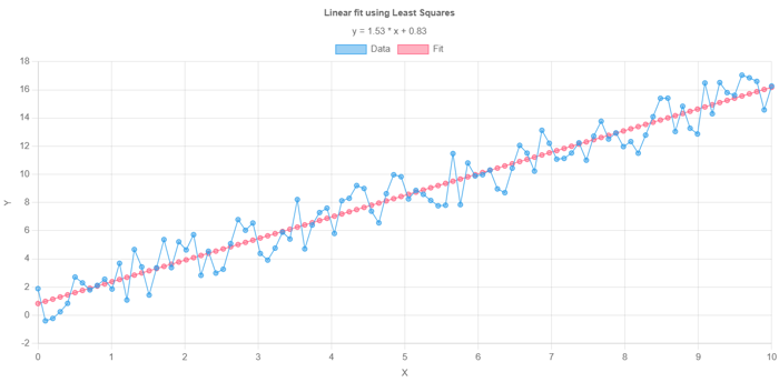
Linear regression analysis of sample data points using COPHASAL matrix operations.
Use of AI
Much of the code for this example was generated with the help of an AI assistant. Of course, I had to check the details and make sure the script ran on COPHASAL. I have found that AI coding assistants can even infer COPHASAL-specific functions and syntax if provided with sufficient context. However, this is not fully reliable yet, so it is important to verify the generated code when using such tools.