Version 1.13.29
The highlight of this release is matrix operations including Solver algorithms that support gradients, however, I will describe these in the next blog post. This post focuses on the new Basic_Cons.lua example script that demonstrates how to set up and use basic lens construction constraints during optimization. These constraints help against virtual ray tracing and beam clipping. Apart from that, there are several updates and additions that improve usability and performance. An issue with reacting parameters that could have caused a crash has also been fixed. Various improvements to reference rays tracing algorithm have been made as well.
Basic Constraints Example
Setting Up Basic_Cons.lua
The script Basic_Cons.lua located in the examples subfolder returns a table of functions. These functions take the Solver object as an argument and add the respective constraints to it. You can capture the script’s return in a local table like local bc = runfile"Basic_Cons". By the way, the function runfile() has been updated to supply optional arguments to the script being run. And the script Basic_Cons accepts a table as an optional argument. So you can also do the following:
local bc = runfile("Basic_Cons", {
    edg = 0.1,      -- minimum edge thickness
    cen = 0.1,      -- minimum center thickness, always along field 1 chief ray
    tol = 0.01,     -- tolerance for constraints
    along_z = true, -- edge thickness along local z axis instead of the marginal ray direction
    sym_yz = true,  -- clearance in the yz-plane instead of the xz-plane
    zoom_pos = 1    -- zoom position to apply constraints at
})
-- Each key in the above table is also optional. Default values are shown.
Interface Functions
The returned table bc contains the following functions:
bc.ZMP(zm_pos) --[[Sets the zoom position to zm_pos, for subsequent tasks.]]

bc.BCI(opt, {1, 2}) --[[
Adds to opt, edge and center thickness constraints for all surfaces,
but ignoring surfaces in the supplied list.
opt: is a Solver
{1, 2} is the list of surfaces to ignore, defaults to an empty list
]]

bc.BCS(opt, {1, 2}) --[[
Adds to opt, edge and center thickness constraints for selected surfaces,
The second argument is the list of surfaces to include and defaults to an empty list
]]

bc.CLR(opt, line_ray_id, line_surface, point_ray_id, point_surface, toggle_sign) --[[
Add to opt, clearance constraint between a line and a point
Line is defined by the ray 'line_ray_id' originating from surface 'line_surface'
Point is defined by the intersection of ray 'point_ray_id' with surface 'point_surface'
line_ray_id and point_ray_id are ray_id tables with optional z field.
toggle_sign is boolean, true will reverse the sign of the constraint.
This constraint uses the sym_yz flag set earlier.
]]
Example
Let us look at an example demonstrating the clearance constraint. The following code snippet realizes a simple reflective system as shown below.
blank()

-- Wavelengths
set("WL W 1", 0.5)
set_pwl(1)

-- Fields
ins_fld(2, {x = 0.0, y = 5.0, vxp = 0.0, vyp = 0.0, vxm = 0.0, vym = 0.0})
ins_fld(3, {x = 0.0, y = -5.0, vxp = 0.0, vyp = 0.0, vxm = 0.0, vym = 0.0})

-- Sequential surfaces
set("THI S 1", 100000000000.0);

set("THI S 2", 15.0);
set_label("S 2", "body")

ins_surf("S 3", {type = "SPHERE", glass = "N-BK7|SCHOTT", rdy = -20.0, thi = -10.0})
set_label("S 3", "m1")
set("REPOS S 'm1'", "BEND", 1)
set("ALPHA S 'm1'", -3, 1)
set("RFR S 'm1'", "REFLECT", 1)

set_stop(2)

-- Variables
vary("ALPHA S 'm1'", 1)
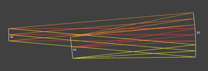
System with beam clipping. Image plane, S4, is clipping rays.
The mirror needs to be tilted further such that the top of the image plane (defined by the intersection of the chief ray from field 2) clears the minus Y marginal ray from field 3 that originates from surface 2. With the tilt about the X axis (ALPHA) of the mirror (S3) as a variable, we can optimize the system to avoid this beam clipping. But before a full optimization, we will setup the Solver with a clearance constraint and perform an evaluation run.
local bc = runfile"Basic_Cons"

local o = Solver.new()
o:set_cost(get_cost)

o:set_max_eval(0)

-- CLR(opt, line_ray_id, line_surface, point_ray_id, point_surface, toggle_sign)
bc.CLR(o, {f=3, r="ym"}, 2, {f=2}, 4, true)

o:solve()
The above code results in the following evaluation output:
Optimizer              : LN_COBYLA
Local Algo             : LN_COBYLA
Dimension              : 1
Cost Function          : user_cost
Inequality Constraints : 1
Equality Constraints   : 0
------ Evaluation Run ------
Cost: 5.206

<= 0 constraints
CLC_L2_P4 : -0.6521

= 0 constraints
----------------------------
Notice that the clearance constraint is named CLC_L2_P4, indicating clearance between ray from surface 2 (L2) and point on surface 4 (P4). The negative value indicates that the constraint is not violated. But we know from the system layout above that the rays are indeed being clipped. So we will rerun the evaluation but this time use false for the last argument of bc.CLR().
...
<= 0 constraints
CLC_L2_P4 : 0.8521
...
Now we run the full optimization with maximum 25 evaluations. Here is the output.
Optimizer              : LN_COBYLA
Local Algo             : LN_COBYLA
Dimension              : 1
Cost Function          : user_cost
Inequality Constraints : 1
Equality Constraints   : 0
------ Evaluation Run ------
Cost: 5.206

<= 0 constraints
CLC_L2_P4 : 0.8521

= 0 constraints
----------------------------
Eval No.:   25, ############ Cost: 17.02
Optimization complete, final cost: 17.022492
------- Final Result -------
Cost: 17.02

<= 0 constraints
CLC_L2_P4 : 8.546e-09

= 0 constraints
----------------------------
Notice that the final value of the clearance constraint is very close to zero, indicating that the rays just clear the image plane edge by a margin defined by the minimum edge thickness parameter. Here is the before and after comparison of the system layout.

System layout before and after optimization with clearance constraint.