Introducing COPHASAL v1.0.0
We are happy to announce the general release of COPHASAL. We would like to express our gratitude to the early adopters of the software for their time and valuable suggestions. This version incorporates many of your suggestions and our Engineering Services’ requirements. The remainder of your suggestions have made it onto our development action items list.
As we march forward, COPHASAL will experience rapid development driven not only by our internal needs but, more importantly, by your continued input. We recommend that you check our blog section regularly, or even better, subscribe to the feed.
Right now, the best way to interface with COPHASAL is by means of scripts. The COPHASAL scripting language is based on the Lua programming language, and the default file extension is also .lua. To edit these scripts, I highly recommend code editors that support Lua syntax highlighting, which includes almost all of them out there. An added bonus would be if the editor has an integrated terminal to run the COPHASAL application in.
Step One
To begin, download and run the installer. You can access the application from the Start Menu—just launch it. When it starts, COPHASAL sets its working folder to the installation folder. I highly recommend that you change the working folder to your home folder. To do this every time COPHASAL starts, edit the user_setup.lua file. To have COPHASAL open this file, issue the command editfile"user_setup".
print "user_setup..."

-- Load the glass catalogs
add_glass_catalog"schott"

-- Listing precisions
set_numeric_precision(4)

-- Better if the path to setup scripts is removed:
del_path "./scripts"

-- Now change working folder to user folder:

-- Method one: hardcoded path
cd "C:/Users/prtkj/Documents"
-- cd "../testing" -- Or a relative path example

-- Method two: using environment variable
-- local user_folder = os.getenv("USERPROFILE") or "C:/Users"
-- cd(user_folder)
As you may have figured out, -- in Lua is the begining of a line comment.
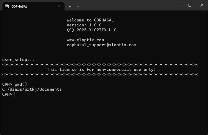
My COPHASAL terminal
Launch the user’s manual by issuing the command help(). This will open the file manual.pdf in the default PDF viewer.
A Singlet Example
Let us open one of the supplied example models, the singlet lens. We will also change the thickness of surface 3 to 2.0 mm.
runfile"singlet"
set("thi s 3", 2.0) -- Set the thickness of surface 3 to 2.0 mm.
s[3].thi = 2.0      -- Same as above, but easier syntax.
-- You can also get parameter values like this:
print(f[2].y) -- Y component of second field.
-- We can use this in an expression as well:
-- f[2].y = f[1].y + 10
showlens() -- Display the YZ section of the model.
Notice the two ways to address the thi parameter (thickness) of the third surface. The second form is more convenient. Currently you can set and get parameter values like this. We plan to add more functionality to this syntax in the future.
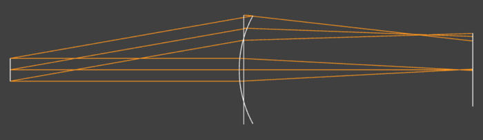
Starting singlet lens
To see the surface listing, issue the command list("s") or simply list"s". This is a Lua feature: when a function expects a single string argument, you don’t have to place the argument in parentheses.
S:
 Z1:     LBL        TYP       RDY          THI          MED          RFR      AUT_APE    COMMENT
 S 1             SPHERE         0        1e+07          AIR     TRANSMIT            0
 S 2             SPHERE         0          100          AIR     TRANSMIT            5
 S 3             SPHERE        50            2    N-BK7|SCH     TRANSMIT        23.68
 S 4             SPHERE         0          100          AIR     TRANSMIT        23.99
 S 5             SPHERE         0            0          AIR     TRANSMIT        16.08
Stop: 2
As you can see, I’ve deliberately shown the virtual ray tracing near the edge, precisely to demonstrate how to address this in the next section.
Constrained Optimization
Before we can optimize, we have to define variables. For this, we will vary both the curvature and thickness of the lens surfaces.
-- Set variables.
vary("thi s 3")
vary("thi s 4")
vary("cuy s 3")
vary("cuy s 4")
Next, we’ll define some functions for constraints. These functions are passed to the optimizer. There are two kinds of constraints: equality and inequality. For inequality constraints, the optimizer always tries to make them negative. We’ll be defining three constraints: one each for the edge thickness, center thickness, and focal length.
-- Define constraint functions.
local function positive_edge()
  local opd = ray_opd({r = "yp", f = 2}, 3) -- OPD of second field, positive y marginal ray, from surface 3 to 4.
  local margin = 0.1 -- 0.1 mm margin.
  return margin - opd -- <= 0 implies opd >= margin.
end

local function positive_thi()
    return 1.0 - s[3].thi -- Thickness of surface 3 must be greater than 1.0 mm.
end

local function efl_constraint()
  local res = first_order()
  return res.F2 - 100.0 -- Focal length of the system must be 100 mm.
end
It’s time to define the optimizer and add these constraints. In COPHASAL, the optimizer is like a variable of the Solver type. You can declare it local to the script or global, pass it as an argument to functions, etc.
-- Define the optimizer.
local o = Solver.new() -- That is the internal optimizer type.

o:set_cost(get_cost)  -- Set the cost function to be the internal one, which is get_cost().
o:set_rel_tol(0.01)   -- Set the relative tolerance to 0.1%.

o:add_ineq(positive_edge, 0.01) -- Add the positive edge constraint with tolerance.
o:add_ineq(positive_thi, 0.01)  -- Add the positive thickness constraint.
o:add_eq(efl_constraint, 0.01)  -- Add the focal length constraint.

o:solve() -- This starts the optmization.
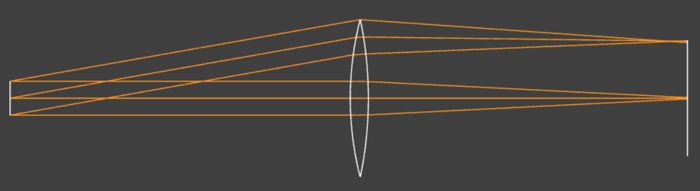
Singlet lens, after optimization
Spot Diagram
Use the spot_data() function to obtain the spot pattern. Then we can scatter plot it.
res = spot_data()
plot(res.spots, {type = "scatter"})
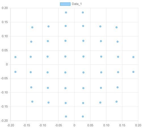
On axis spot pattern on the image surface
Ray Listing
Let us list the ray infomation for the positive Y marginal ray of the second field, using the list_ray() function.
CPH> list_ray({r = "yp", f = 2})
SUR  X          Y          Z          L          M          GPH        T,R        A
S 2  0          5          0          0          0.1736     0.8685     1          -
S 3  0          23.14      2.891      0          0.1736     105.4      0.9458     1
S 4  0          23.14      -2.359     0          0.02468    105.5      0.9528     1
S 5  0          16.37      0          0          -0.07025   201.9      -          1
Intensity transfer: 0.9012
Jones vector: Yamp/Xamp: 0, Yphi-Xphi: 0
Notice that there’s no listing for surface 1. This is because the object is far away, and in such cases, COPHASAL starts the rays from the next surface. The “GPH” column represents the geometric phase, accounting for the index of refraction. It looks like our positive edge thickness constraint just made it.
Final Note
I chose to demo the optimizer for two reasons. First, it demonstrates the capability and flexibility of the COPHASAL scripting environment. You can, for example, pass the solver object to another function as an argument, and that function can populate the solver with all the basic construction constraints. I’ve found the Lua-based scripting to be very easy to manage and flexible at the same time, and with the various coding assistants available these days, it’s also fun.
The second reason is to point out that the optimizer continues to be developed. Expect more updates on this aspect. For this first version, enough functionality has been implemented to help COPHASAL deal with most optical design situations. However, more analysis functionality and interface enhancements will be added regularly. Please stay tuned.
COPHASAL development is primarily driven by internal and external customer requirements. Please write to us if you’d like a feature added or if you discover incorrect behavior. I hope you have success using COPHASAL.